The Latent Space of a Cell: Single-Cell RNA-seq From Droplet to Map

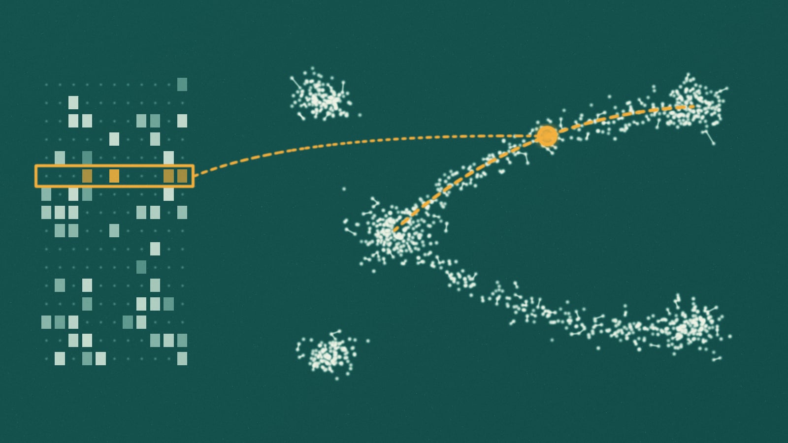
Every cell in your body carries the same genome, yet a neuron and a white blood cell are different machines. The difference is which of its roughly 20,000 protein-coding genes each one is using. Single-cell RNA sequencing reads that difference one cell at a time, by counting the messenger RNA copies of each gene inside it. What comes out is a table: one row per cell, one column per gene, and a count in every entry.

Read a row as coordinates and each cell becomes a point in a space with tens of thousands of dimensions. Almost all of that space is empty. Genes work in programs that rise and fall together, so real cells crowd onto a much smaller surface inside it, and the central job of single-cell analysis is to find that surface: a latent space where nearby points are cells in similar states. The colorful maps of islands that open nearly every single-cell paper are the last step of that search, a flat picture of a curved object. Our article on protein and DNA language models charted the latent space of sequences. This one charts the latent space of cells.

The data is no longer small. One of the first single-cell RNA sequencing experiments, published in 2009, read a single cell from an early mouse embryo; the CZ CELLxGENE Census, a public collection of standardized datasets, held about 120 million unique human and mouse cells in its November 2025 release. Below, you will run the standard pipeline in your browser, meet scVI, a variational autoencoder whose latent space is the map, and measure what a 2D picture keeps. Then come the foundation models trained on tens of millions of cells, and the simple baselines that keep beating them.

How a cell becomes 20,000 numbers

The trick that made single-cell sequencing scale is a barcode. In a droplet experiment, a tissue is broken into a suspension of single cells, which flow through a microfluidic chip alongside tiny gel beads. Oil pinches the stream into droplets, and the cells are dilute enough that a droplet rarely holds more than one. Every primer on a bead carries the same cell barcode, a short DNA sequence unique to that bead, plus a random tag called a unique molecular identifier, or UMI, that differs from primer to primer. Inside the droplet, the cell's messenger RNA is copied into DNA and every copy is stamped with both. Then the droplets are broken, and everything is pooled and sequenced together.

from tissue to a count matrix

1. dissociate the tissuea suspension of single, living cells
2. microfluidic chip
   one cell and one bead per dropletevery primer on a bead shares one cell barcode and has its own random UMI
3. tag every moleculeeach mRNA is copied into DNA carrying the cell barcode and a UMI

   [cell barcode][UMI][poly-T] + mRNA

4. break the droplets
   pool and sequencemillions of reads from thousands of cells in one run
5. map reads to genes
   count matrixcells by genes; reads that share a UMI count once

Afterwards, the barcode says which cell a read came from, and the UMI says which original molecule. Amplification copies some molecules far more often than others, so counting distinct UMIs instead of reads removes most of that distortion. Drop-seq, one of the first droplet methods, profiled 44,808 mouse retinal cells in 2015 and found 39 distinct populations. Two years later the commercial version from 10x Genomics profiled 68,000 blood cells, and the company released a dataset of 1.3 million mouse brain cells.

The result is a count matrix, and it is mostly zeros. A cell holds hundreds of thousands of mRNA molecules and a droplet captures only a fraction of them, so weakly expressed genes are often missed; in typical datasets more than 90 percent of entries are zero. For years these zeros were called dropouts and modeled as a separate failure. Valentine Svensson showed in 2020 that for droplet data with UMIs they are about what sampling a few molecules from a negative binomial distribution predicts, with no extra inflation needed. A zero mostly means not sampled, rather than not expressed.

The standard single-cell pipeline, step by step

Most analyses run the same sequence of steps, implemented in tools such as Scanpy in Python and Seurat in R. Each step removes one kind of noise or answers one question.

the standard analysis

1. 1

   quality controldrop empty droplets, doublets, and dying cells with many mitochondrial reads
2. 2

   normalizedivide by each cell's total, scale to 10,000, take log(1 + x)
3. 3

   select geneskeep the 2,000 or so genes that vary most between cells
4. 4

   PCAcompress to 30 to 50 components
5. 5

   neighbor graphconnect each cell to its 15 or so nearest neighbors
6. clusterLeiden finds communities in the graph

   mapUMAP or t-SNE draws the graph in 2D
7. 7

   annotatemarker genes put names on the clusters

Three of these steps deserve a closer look.

Normalization handles library size. One droplet may catch 1,000 molecules and the next 10,000 from the same kind of cell, by chance. Dividing by the total and taking a log puts cells on a common scale; skip it, and the largest axis of variation is sequencing depth, not biology.

PCA is a denoiser as much as a compressor. Measurement noise is spread thinly across every direction, while biological programs move many genes together and concentrate in a few directions. Keeping the top 30 to 50 components keeps most of the biology and drops most of the noise.

The neighbor graph is the real latent structure. Clustering and the 2D map are both computed from it. Leiden, the standard clustering algorithm, finds communities of cells more connected to each other than to the rest. It fixed a flaw in its predecessor, Louvain, which in the Leiden authors' tests left up to 16 percent of communities internally disconnected.

The sandbox below runs this pipeline on 1,200 simulated cells from six types, in which progenitors turn continuously into two fates, the way blood progenitors become red cells or platelet-making megakaryocytes. Leiden is not available in the browser's Python, so spectral clustering on the same kind of 15-neighbor graph stands in; unlike Leiden, it has to be told how many clusters to find.

1import numpy as np
2import matplotlib.pyplot as plt
3from sklearn.decomposition import PCA
4from sklearn.cluster import SpectralClustering
5from sklearn.manifold import TSNE
6from sklearn.metrics import adjusted_rand_score
7 
8rng = np.random.default_rng(11)
9NORMALIZE = True        # set to False and rerun
10 
11# --- Simulate a droplet experiment -----------------------------------
12# 1,200 cells and 2,000 genes. Each of six cell types switches on its
13# own program of 40 genes; progenitors turn into erythroid cells or
14# megakaryocytes along a continuum.
15n_cells, n_genes = 1200, 2000
16names = ["T cell", "B cell", "monocyte", "progenitor", "erythroid", "megakaryocyte"]
17base = rng.lognormal(-1.5, 1.6, n_genes)             # baseline expression
18prog = np.ones((6, n_genes))
19for k in range(6):
20    prog[k, rng.choice(n_genes, 40, replace=False)] = rng.uniform(4, 12, 40)
21 
22truth = rng.choice(6, n_cells, p=[0.2, 0.15, 0.15, 0.15, 0.2, 0.15])
23s = rng.uniform(0, 1, n_cells)                       # how far along a branch
24mu = np.empty((n_cells, n_genes))
25for i, k in enumerate(truth):
26    if k < 4:                                        # a settled state
27        mu[i] = base * prog[k]
28    else:                                            # on a branch: progenitor to fate
29        mu[i] = base * ((1 - s[i]) * prog[3] + s[i] * prog[k])
30truth[(truth > 3) & (s < 0.15)] = 3                  # early cells still look like progenitors
31 
32# Each droplet catches a different number of molecules (library size),
33# and counts are gamma-Poisson (negative binomial) samples around that.
34library = rng.lognormal(np.log(2000), 0.5, n_cells)
35mean = mu / mu.sum(1, keepdims=True) * library[:, None]
36X = rng.poisson(rng.gamma(2.0, mean / 2.0))
37print(f"count matrix: {n_cells} cells x {n_genes} genes")
38print(f"zeros: {100 * (X == 0).mean():.0f}% of entries")
39print(f"molecules per cell: {X.sum(1).min()} to {X.sum(1).max()}")
40 
41# --- The standard pipeline -------------------------------------------
42if NORMALIZE:
43    Xn = np.log1p(X / X.sum(1, keepdims=True) * 1e4)  # counts per 10k, then log
44else:
45    Xn = np.log1p(X)
46m, v = Xn.mean(0), Xn.var(0)
47hvg = np.argsort(v / (m + 0.1))[-400:]                # most variable genes
48pcs = PCA(30, random_state=0).fit_transform(Xn[:, hvg])
49# Spectral clustering on a 15-nearest-neighbor graph stands in for Leiden.
50clusters = SpectralClustering(6, affinity="nearest_neighbors", n_neighbors=15,
51                              random_state=0).fit_predict(pcs)
52emb = TSNE(perplexity=30, init="pca", random_state=0).fit_transform(pcs)
53 
54depth = np.corrcoef(pcs[:, 0], np.log(X.sum(1)))[0, 1]
55print(f"PC1 vs sequencing depth: r = {depth:+.2f}")
56print(f"clusters vs true cell types: ARI = {adjusted_rand_score(truth, clusters):.2f}  (1.0 is perfect)")
57 
58# Color each cluster like the true type most of its cells belong to.
59major = {c: np.bincount(truth[clusters == c]).argmax() for c in np.unique(clusters)}
60 
61fig, axes = plt.subplots(1, 3, figsize=(15, 4.6))
62for ax, xy, title in [(axes[0], pcs[:, :2], "first two PCs, true types"),
63                      (axes[1], emb, "t-SNE map, true types")]:
64    for k in range(6):
65        ax.scatter(*xy[truth == k].T, s=6, color=f"C{k}", label=names[k])
66    ax.set_title(title)
67for c, k in major.items():
68    axes[2].scatter(*emb[clusters == c].T, s=6, color=f"C{k}",
69                    label=f"cluster {c}: mostly {names[k]}")
70axes[2].set_title("t-SNE map, graph clusters")
71for ax in axes:
72    ax.set_xticks([]); ax.set_yticks([])
73axes[0].legend(fontsize=8, markerscale=2)
74axes[2].legend(fontsize=7, markerscale=2)
75plt.tight_layout()
76plt.show()
77 

The clusters recover the true types with an adjusted Rand index around 0.8, and the disagreements sit where progenitors turn into erythroid cells and megakaryocytes: a continuum has no natural border, and clustering draws one anyway. The left panel shows why the pipeline keeps 30 components. The first two separate T cells and monocytes and pile everything else into one heap.

Now set NORMALIZE to False and rerun. The first principal component now tracks how many molecules each droplet caught, with a correlation around 0.96, and the clusters get worse. (This toy keeps 2,000 genes and is about two thirds zeros; full matrices are sparser.)

A latent space that knows about counts: scVI

PCA is linear and implicitly treats noise as Gaussian. Counts are neither. scVI (single-cell variational inference), published in 2018 by Romain Lopez, Nir Yosef, Michael Jordan and colleagues at Berkeley, replaces PCA with a variational autoencoder built for counts.

It starts from a generative story. Each cell has a latent state $z$, 10 numbers drawn from a standard normal distribution, and a library size $\ell$ that absorbs how many molecules its droplet happened to catch. A decoder network turns $z$, together with the cell's batch label $s$, into the share of the cell's molecules that each gene should receive. The observed counts are drawn around that:

$$z_n \sim \mathcal{N}(0, I), \qquad x_{ng} \sim \mathrm{NB}\big(\ell_n \, \rho_g(z_n, s_n),\ \theta_g\big)$$

Here $\rho_g$ is the decoder's share for gene $g$ and $\theta_g$ sets how overdispersed its counts are. An encoder network learns to run the story backwards, from counts to a distribution over $z$, and both networks train together by variational inference. (The original paper added a zero-inflation term; scvi-tools, the library that grew out of it, also offers the plain negative binomial that Svensson's analysis suggests is enough.)

scVI, one cell at a time

1. counts for one cellthousands of genes, mostly zeros
2. encoder networkoutputs a distribution, not a single point
3. latent state z10 numbers: what the cell is

   library sizehow many molecules were caught

   batch labelwhich lab, run, or chemistry; given, not learned
4. decoder networkexpected share of molecules for every gene
5. negative binomial likelihoodhow well the expected counts explain the observed ones

The design choice that matters most is where the batch label goes. Cells of the same type look different when processed in different labs, on different days, or with different chemistry. Because the decoder is told the batch, the cheapest way to reconstruct the counts is to keep $z$ about biology and let the decoder add each batch's distortion. Batch correction falls out of the architecture. And because training runs on minibatches, it scales: the authors trained it on up to a million cells from the 1.3 million cell mouse brain dataset, in under an hour with early stopping.

It held up in testing. A 2022 benchmark led by Malte Luecken and Fabian Theis compared 68 method and preprocessing combinations on more than 1.2 million cells across 13 integration tasks, and scANVI (a sibling of scVI that also uses known cell labels), scVI, Scanorama and scGen performed well, particularly on the hardest tasks. The latent space scVI learns is a working coordinate system for cell state: you cluster in it, compare groups of cells through the decoder, and follow processes such as differentiation as paths through it.

What a 2D map keeps, and what it throws away

Neither 10 latent dimensions nor 50 principal components can be looked at. t-SNE (2008) and UMAP (2018, popularized in single-cell work by a 2019 Nature Biotechnology paper) squash the neighbor structure into two dimensions, pulling cells that are close in the high-dimensional space together on the page and pushing the rest apart. Neither was built to preserve distances, and in two dimensions they cannot.

The sharpest case against them came in 2023 from Tara Chari and Lior Pachter, in "The specious art of single-cell genomics." By the Johnson-Lindenstrauss lemma, keeping every pairwise distance within 20 percent for just 10,000 cells needs at least 1,842 dimensions. In real datasets, comparing each cell's 30 nearest neighbors on the map with its 30 nearest in the original space gave an average Jaccard distance above 0.7: fewer than half of a cell's neighbors on the map were true neighbors. As a provocation, they built Picasso, an autoencoder that forces data into an arbitrary shape such as an elephant, and found that the elephant scored about as well as UMAP and t-SNE on their measures of how well distances between and within cell types survive.

Jan Lause, Philipp Berens and Dmitry Kobak replied in 2024 with "The art of seeing the elephant in the room." They reproduced the elephant result, then pointed out that both measures only test distance preservation, where 2D PCA wins by construction. On what biologists actually read from a map, whether neighbors and cell types are preserved and whether known types separate, t-SNE and UMAP clearly beat both the elephant and PCA. The maps do not preserve distances, they concluded, but still carry biologically relevant information.

Both sides are right about different things, and you can measure both. The sandbox below places eight cell types in a 30-dimensional latent space, draws three 2D maps, and scores each one twice: the share of each cell's 15 nearest neighbors that survive (local structure), and how well distances between cell-type centers survive (global structure).

1import numpy as np
2import matplotlib.pyplot as plt
3from sklearn.decomposition import PCA
4from sklearn.manifold import TSNE
5from sklearn.neighbors import NearestNeighbors
6 
7rng = np.random.default_rng(5)
8 
9# --- Cells in a 30-dimensional latent space --------------------------
10# Eight cell types. Their centers sit at known distances from each
11# other, so we can check whether a 2D map keeps those distances.
12n_types, per_type, d = 8, 120, 30
13centers = rng.normal(0, 1, (n_types, d)) * rng.uniform(2, 6, (n_types, 1))
14Z = np.vstack([c + rng.normal(0, 1, (per_type, d)) for c in centers])
15types = np.repeat(np.arange(n_types), per_type)
16 
17def neighbor_recall(high, low, k=15):
18    """Share of each cell's k nearest neighbors that survive in the map."""
19    nh = NearestNeighbors(n_neighbors=k + 1).fit(high).kneighbors(high, return_distance=False)[:, 1:]
20    nl = NearestNeighbors(n_neighbors=k + 1).fit(low).kneighbors(low, return_distance=False)[:, 1:]
21    return np.mean([len(set(a) & set(b)) / k for a, b in zip(nh, nl)])
22 
23def center_distance_corr(high, low):
24    """Do distances between cell-type centers survive in the map?"""
25    ch = np.array([high[types == t].mean(0) for t in range(n_types)])
26    cl = np.array([low[types == t].mean(0) for t in range(n_types)])
27    iu = np.triu_indices(n_types, 1)
28    dh = np.linalg.norm(ch[:, None] - ch[None], axis=-1)[iu]
29    dl = np.linalg.norm(cl[:, None] - cl[None], axis=-1)[iu]
30    return np.corrcoef(dh, dl)[0, 1]
31 
32maps = {
33    "PCA, 2D": PCA(2).fit_transform(Z),
34    "t-SNE, perplexity 5": TSNE(perplexity=5, init="pca", random_state=0).fit_transform(Z),
35    "t-SNE, perplexity 50": TSNE(perplexity=50, init="pca", random_state=0).fit_transform(Z),
36}
37 
38fig, axes = plt.subplots(1, 4, figsize=(17, 4.2), gridspec_kw={"width_ratios": [1, 1, 1, 1.25]})
39scores = {}
40for ax, (name, xy) in zip(axes, maps.items()):
41    scores[name] = (neighbor_recall(Z, xy), center_distance_corr(Z, xy))
42    ax.scatter(xy[:, 0], xy[:, 1], c=types, cmap="tab10", s=5)
43    ax.set_title(name); ax.set_xticks([]); ax.set_yticks([])
44 
45y = np.arange(len(scores))
46ax = axes[3]
47ax.barh(y - 0.2, [v[0] for v in scores.values()], 0.4, label="neighbors kept (local)")
48ax.barh(y + 0.2, [v[1] for v in scores.values()], 0.4, label="center distances kept (global)")
49ax.set_yticks(y); ax.set_yticklabels(list(scores)); ax.invert_yaxis()
50ax.set_xlim(0, 1); ax.legend(fontsize=8, loc="lower right")
51ax.set_title("what each map keeps")
52plt.tight_layout()
53plt.show()
54 
55for name, (local, glob) in scores.items():
56    print(f"{name:22s} neighbors kept {local:.0%}   center distance correlation {glob:+.2f}")
57 

PCA keeps the global picture, with a correlation above 0.9, but fewer than one in five of each cell's neighbors. t-SNE keeps about twice as many neighbors and loses most of the global picture. At perplexity 50 the same cell types shrink to tight dots: the size of an island on a map is a setting, not a measurement. Now change init="pca" to init="random" in both t-SNE calls and rerun, and the global correlation falls to around zero. Kobak and George Linderman showed in 2021 that this explains most of UMAP's reputation for better global structure: it comes largely from UMAP's default initialization, and t-SNE given the same informative start does about as well.

That leaves some practical rules for reading a single-cell map:

• Trust neighborhoods and clusters, and confirm them with marker genes.
• Do not read distances between islands, island sizes, or the empty space between them.
• Do quantitative work in the higher-dimensional space, whether that is PCA or a latent space like scVI's, and use the map to look.

Single-cell foundation models: a cell as a sentence

Large language models learn from unlabeled text, and single-cell atlases are an enormous unlabeled corpus. The obstacle to pretraining a transformer on them is that a cell is not a sentence: its genes come with counts, not an order.

Geneformer (Christina Theodoris and colleagues, Nature, 2023) solved that with a ranking. Pretrained on about 30 million transcriptomes, it writes each cell as its genes sorted from most to least expressed, after scaling each gene by its typical level across the corpus, and learns to predict genes hidden from that list. Fine-tuned with little labeled data, it improved predictions on network biology tasks, and simulated gene deletions inside the model pointed to candidate therapeutic targets for cardiomyopathy.

scGPT (Nature Methods, 2024), pretrained on more than 33 million cells with tokens that pair each gene with a binned expression value, reported strong results on cell type annotation, batch integration, gene network inference, and predicting how cells respond to genetic perturbations.

That last task is the prize. A model that predicts what happens when you knock down a gene or add a drug, in an experiment nobody has run, would be a virtual cell: a way to screen thousands of interventions before anyone opens a freezer.

The baselines bite back

The first careful tests were sobering. In 2025, Kasia Kedzierska and colleagues at Oxford and Microsoft Research tested scGPT and Geneformer zero-shot, using their embeddings without fine-tuning, as you would in discovery work where nobody knows the cell types yet. At separating known cell types, both did worse than simply selecting highly variable genes, and worse than Harmony and scVI. In batch integration, Geneformer ranked last, its embeddings more organized by batch than the original data. scGPT had real wins on one blood dataset and on complex integration tasks, but those tasks used datasets from its own pretraining corpus.

Perturbation prediction fared no better. Constantin Ahlmann-Eltze, Wolfgang Huber and Simon Anders pitted five foundation models (scGPT, scFoundation, Geneformer, scBERT and UCE) and two other deep learning models (GEARS and CPA) against deliberately simple baselines. For combinations they used a CRISPR activation experiment in a leukemia cell line that switched on 100 single genes and 124 pairs.

Task	Simple baseline	Result
Predict switching on two genes at once	Add the two single-gene effects	Every deep model had substantially higher error
Find gene pairs that interact surprisingly	Predict no change	No model beat it
Predict a knockdown never seen in training	The average training effect, or a linear model	No deep model consistently beat either

The details sharpen the point. A plain linear model given scGPT's or scFoundation's gene embeddings did as well as or better than those models with their own decoders. The only approach that consistently beat everything was a linear model with perturbation embeddings learned from a different perturbation experiment, in another cell line. Atlas pretraining, the authors concluded, gave only a small benefit over random embeddings, while pretraining on perturbation data helped.

In 2025 the Arc Institute ran the first Virtual Cell Challenge, in which more than 1,200 teams submitted predictions of how cells respond to gene knockdowns. Arc's own lesson starts with scoring: no single metric captures model quality, and a narrow one invites optimizing the metric instead of the biology. The 2026 edition, with final submissions due November 5, is zero-shot: teams predict knockdown responses in six cell lines with no challenge-specific training set.

One counterpoint: a February 2026 preprint from GenBio AI, not yet peer reviewed, evaluated more than 600 models and found that some foundation model embeddings do significantly beat simple baselines. But the best single source was interactome knowledge, networks of which genes and proteins interact, such as STRING. Single-cell foundation models like scGPT beat a PCA baseline and still trailed it.

Read together, the results suggest a pattern. What predicts a perturbation's effect is information about how genes act on each other, from perturbation experiments or interaction networks. Tens of millions of snapshots of cells at rest carry less of it than hoped, because watching a system is not the same as pushing on it.

What this does and does not show

A cluster is a choice. Leiden's resolution setting decides how many clusters you get, and continuous processes get cut into pieces whatever you choose, as the first sandbox shows. Clusters become cell types only when marker genes and biology back them up.

A map is a sketch. 2D embeddings keep useful neighborhoods and separate known types. They do not keep distances, sizes, or gaps, and no setting fixes that in two dimensions.

The baselines are not the ceiling. These are results about current models on current benchmarks. Perturbation datasets cover a handful of cell lines and the metrics are contested. Ahlmann-Eltze and colleagues called a general model of cell state still elusive, which is a statement about today.

Overlap cuts both ways. Pretraining corpora now overlap many evaluation datasets, so a strong score can mean the model has seen the test. Some of scGPT's best zero-shot results came on data from its own pretraining set.

Takeaways

Single-cell RNA-seq turns each cell into a sparse vector of molecule counts, with barcodes and UMIs tracing every molecule to its cell. The standard pipeline normalizes for library size, compresses with PCA, connects cells into a neighbor graph, and reads clusters and maps off that graph. scVI swaps the linear step for a variational autoencoder built for counts, and by giving the batch label to its decoder it learns a latent space where batch effects mostly disappear.

The 2D maps everyone publishes keep neighborhoods and separate cell types, and cannot keep distances, so the gaps and island sizes on a UMAP mean little. The debate over whether those maps are specious is, underneath, a debate about what a map is for.

Foundation models trained on tens of millions of cells have so far struggled to beat simple baselines, from zero-shot clustering to predicting perturbations, and the most consistent signal is that knowing how genes act on each other matters more than observing more cells. Charting the latent space of a cell works like charting any latent space: the map is only as good as what the data can reveal, and no model can invent an experiment nobody ran.

Frequently asked questions

What is single-cell RNA sequencing?

It measures which genes each individual cell is expressing by counting the messenger RNA molecules inside it. In droplet methods, each cell is sealed in a droplet with a bead whose primers carry a cell barcode and a unique molecular identifier, so after pooled sequencing every molecule can be traced to its cell and counted once. The output is a matrix of cells by genes, mostly zeros.

What is scVI?

scVI (single-cell variational inference) is a variational autoencoder for single-cell counts, published by Lopez and colleagues in 2018. It encodes each cell into a 10-dimensional latent state, decodes that state together with the batch label into expected counts under a negative binomial model, and is trained by variational inference. Because the decoder handles batch effects, the latent space is largely batch corrected, and training scales to a million cells.

Are UMAP and t-SNE plots misleading?

They mislead if you read distances off them. Two dimensions cannot preserve the distances between thousands of cells, and Chari and Pachter found that on typical maps, more than half of a cell's 30 nearest neighbors are not its true neighbors. But Lause, Berens and Kobak showed the maps still preserve neighborhoods and separate cell types far better than an arbitrary shape. Read clusters and neighborhoods from them, not gaps, sizes, or distances between islands.

Why run PCA before clustering and UMAP?

PCA removes noise. Measurement noise is spread across all genes, while biological programs move many genes together and concentrate in a few principal components. Keeping the top 30 to 50 components keeps most of the biology, makes the nearest neighbor graph more reliable, and makes everything after it faster.

Do single-cell foundation models beat simple baselines?

Not yet, on the tasks tested most carefully. In zero-shot cell type clustering, scGPT and Geneformer did worse than selecting highly variable genes. In predicting the effects of genetic perturbations, five foundation models failed to beat deliberately simple linear baselines. A 2026 preprint found that some embeddings do help, but the best came from gene interaction networks rather than from single-cell atlases.

References

1. Tang, F., Barbacioru, C., Wang, Y., Nordman, E., Lee, C., Xu, N., et al., and Surani, M. A. (2009). "mRNA-Seq whole-transcriptome analysis of a single cell." Nature Methods 6(5):377-382. DOI

2. Islam, S., Zeisel, A., Joost, S., La Manno, G., Zajac, P., Kasper, M., Lönnerberg, P., and Linnarsson, S. (2014). "Quantitative single-cell RNA-seq with unique molecular identifiers." Nature Methods 11(2):163-166. DOI

3. Macosko, E. Z., Basu, A., Satija, R., Nemesh, J., Shekhar, K., Goldman, M., et al., and McCarroll, S. A. (2015). "Highly parallel genome-wide expression profiling of individual cells using nanoliter droplets." Cell 161(5):1202-1214. DOI

4. Zheng, G. X. Y., Terry, J. M., Belgrader, P., Ryvkin, P., Bent, Z. W., Wilson, R., et al., and Bielas, J. H. (2017). "Massively parallel digital transcriptional profiling of single cells." Nature Communications 8:14049. DOI

5. CZ CELLxGENE Discover. "Census data releases" (long-term supported release of 2025-11-08). Documentation

6. Svensson, V. (2020). "Droplet scRNA-seq is not zero-inflated." Nature Biotechnology 38(2):147-150. DOI

7. Wolf, F. A., Angerer, P., and Theis, F. J. (2018). "SCANPY: large-scale single-cell gene expression data analysis." Genome Biology 19:15. DOI

8. Traag, V. A., Waltman, L., and van Eck, N. J. (2019). "From Louvain to Leiden: guaranteeing well-connected communities." Scientific Reports 9:5233. DOI

9. Lopez, R., Regier, J., Cole, M. B., Jordan, M. I., and Yosef, N. (2018). "Deep generative modeling for single-cell transcriptomics." Nature Methods 15(12):1053-1058. DOI

10. Luecken, M. D., Büttner, M., Chaichoompu, K., Danese, A., Interlandi, M., Mueller, M. F., et al., and Theis, F. J. (2022). "Benchmarking atlas-level data integration in single-cell genomics." Nature Methods 19(1):41-50. DOI

11. van der Maaten, L. and Hinton, G. (2008). "Visualizing data using t-SNE." Journal of Machine Learning Research 9:2579-2605. Paper

12. McInnes, L., Healy, J., and Melville, J. (2018). "UMAP: Uniform Manifold Approximation and Projection for Dimension Reduction." arXiv:1802.03426. arXiv

13. Becht, E., McInnes, L., Healy, J., Dutertre, C.-A., Kwok, I. W. H., Ng, L. G., Ginhoux, F., and Newell, E. W. (2019). "Dimensionality reduction for visualizing single-cell data using UMAP." Nature Biotechnology 37(1):38-44. DOI

14. Chari, T. and Pachter, L. (2023). "The specious art of single-cell genomics." PLOS Computational Biology 19(8):e1011288. DOI

15. Lause, J., Berens, P., and Kobak, D. (2024). "The art of seeing the elephant in the room: 2D embeddings of single-cell data do make sense." PLOS Computational Biology 20(10):e1012403. DOI

16. Kobak, D. and Linderman, G. C. (2021). "Initialization is critical for preserving global data structure in both t-SNE and UMAP." Nature Biotechnology 39(2):156-157. DOI

17. Kobak, D. and Berens, P. (2019). "The art of using t-SNE for single-cell transcriptomics." Nature Communications 10:5416. DOI

18. Theodoris, C. V., Xiao, L., Chopra, A., Chaffin, M. D., Al Sayed, Z. R., Hill, M. C., et al., and Ellinor, P. T. (2023). "Transfer learning enables predictions in network biology." Nature 618(7965):616-624. DOI

19. Cui, H., Wang, C., Maan, H., Pang, K., Luo, F., Duan, N., and Wang, B. (2024). "scGPT: toward building a foundation model for single-cell multi-omics using generative AI." Nature Methods 21(8):1470-1480. DOI

20. Kedzierska, K. Z., Crawford, L., Amini, A. P., and Lu, A. X. (2025). "Zero-shot evaluation reveals limitations of single-cell foundation models." Genome Biology 26:101. DOI

21. Ahlmann-Eltze, C., Huber, W., and Anders, S. (2025). "Deep-learning-based gene perturbation effect prediction does not yet outperform simple linear baselines." Nature Methods 22(8):1657-1661. DOI

22. Arc Institute (2026). "The 2026 Virtual Cell Challenge: predicting perturbation responses in cell contexts a model has never seen." Announcement

23. Cole, E., Huizing, G.-J., Addagudi, S., Ho, N., Hasanaj, E., Kuijs, M., et al., and Xing, E. P. (2026). "Foundation Models Improve Perturbation Response Prediction." bioRxiv preprint. DOI